[3DGS] 3D Gaussian Splatting for Real-Time Radiance Field Rendering : Paper Review
Paper Information
SIGGRAPH 2023
- title : 3D Gaussian Splatting for Real-Time Radiance Field Rendering
- journal : ACM Transactions on Graphics
- author : Kerbl, Bernhard and Kopanas, Georgios and Leimkhler, Thomas and Drettakis, George

https://repo-sam.inria.fr/fungraph/3d-gaussian-splatting/
3D Gaussian Splatting for Real-Time Radiance Field Rendering
[Müller 2022] Müller, T., Evans, A., Schied, C. and Keller, A., 2022. Instant neural graphics primitives with a multiresolution hash encoding [Hedman 2018] Hedman, P., Philip, J., Price, T., Frahm, J.M., Drettakis, G. and Brostow, G., 2018. Deep blending
repo-sam.inria.fr
Abstract
- Previous Problem :
Achieving high visual quality for Radiance Field Rendering is expensive. - Solution : Three key elements
1. 3D Gaussian
2. interleaved optimization density control
3. a fast visibility-aware rendering algorithm - Result :
1. SOTA visual quality
2. real-time rendering
1. Introduction
(1) 3D Scene representations
Meshes and points : 3D scene representations
(2) NeRF(Neural Radiance Field)
1. Core Concept
- Based on continuous scene representations
- Utilize MLP optimization with volumetric ray-marching
- Perform novel-view synthesis of captured scenes
2. Efficient Radiance Field Solutions
- Rely on continuous representations
- Improve computational efficiency by interpolating stored values
3. Key Approaches
- Voxel grids [Fridovich-Keil and Yu et al., 2022]
- Hash grids [Müller et al., 2022]
- Point-based representations [Xu et al., 2022]
4. Disadvantages
- Stochastic sampling for rendering is costly
- Can result in noise
(3) 3D Guassian (Proposed in this paper)
1. method : 3D gaussian representation
2. goal
- allow real-time rendering for scenes captured with multiple photos
- SOTA visual quality for 1080p and competitive training time
3. three main components
- 3D Guassian
- optimization control
- fast GPU sorting algorithm
4. result
- first real-time rendering with high quality
3. Overview
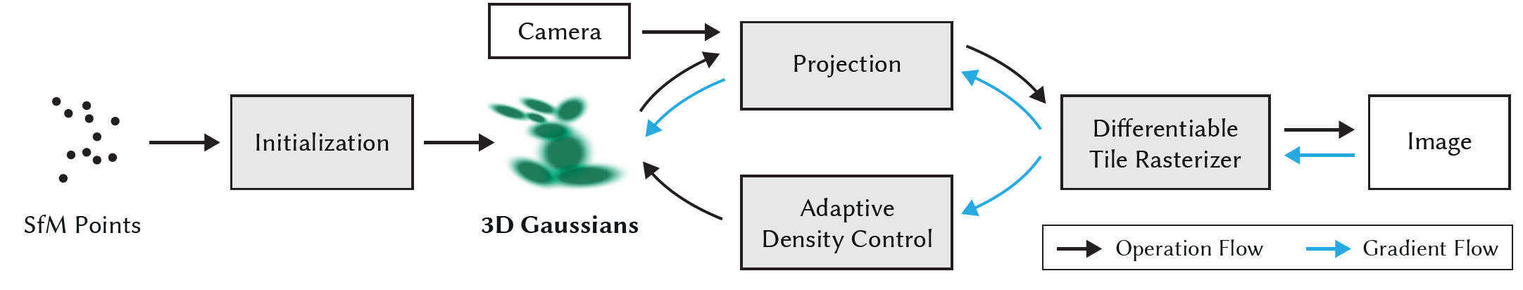
4. Differentiable 3D guassian splatting
goal : optimize a scene representation that allows high-quality novel view synthesis
=> apply differentiable 3D guassian
Previous methods : start from a sparse set of(SfM) points + need normals.
=> it's hard to estimate normals and optimizing noisy normals is challenging
3DGS starts from a sparse set of(SfM) points without normals. (You can see from the equation below that the normal is not used.) // Appendix 1
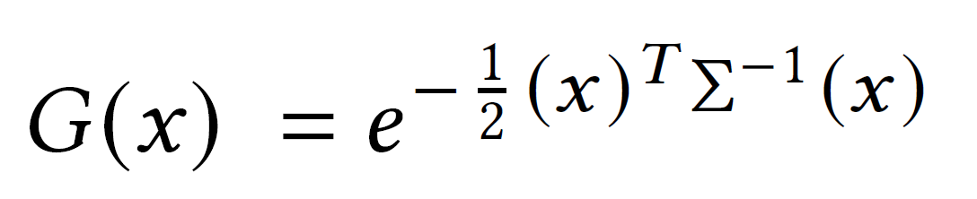
∑ : a full 3D covariance matrix (world space) // Appendix 2
µ = 0 (centered at point)
For 2D rendering, we have to project 3D gaussian onto 2D using the viewing transformation W. To do this, we can transform the covariance matrix from world space to camera space.
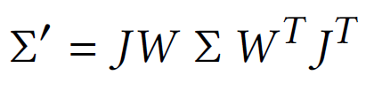
∑' : covariance matrix (camera space)
J : Jacobian of the affine approximation // Appendix 3
The covariance matrix ∑ of a 3D gaussian is analogous to describing the configuation of an ellipsoid.
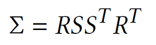
S : Scaling matrix
R : Rotating matrix
Appendix 1 : Additional description of Gaussian function (Korean)
2025.02.07 - [Computer Science/AI] - [3DGS] Gaussian function - 1D gaussian
[3DGS] Gaussian function - 1D gaussian
최근 화제가 되고 있는 Gaussian Splatting에 대해 공부하면서 Gaussian에 대한 수학적인 이해가 부족하다는 것을 느꼈다. 본격적으로 관련 분야를 공부하고 싶기 때문에 수식적으로 꼼꼼하게 공부하고
mobuk.tistory.com
2025.02.07 - [Computer Science/AI] - [3DGS] gaussian function - N-dim gaussian
[3DGS] gaussian function - N-dim gaussian
Contents1D gaussian (1편 - 아래 링크 참조) gaussian function gaussian integralN-Dim gaussian 2D gaussian3D gaussian 2025.02.07 - [Computer Science/AI] - [3DGS] Gaussian function - 1D gaussian [3DGS] Gaussian function - 1D gaussian최근 화제
mobuk.tistory.com
Appendix 2 : Covariance Matrix (TBU)
Appendix 3 : Jacobian Matrix (TBU)
In a nutshell, Jacobian Matrix is the matrix of all its first-order partial derivatives.
5. Opitmization with adaptive density control of 3D gaussians
5.1. Optimization
Optimization is based on successive iterations of rendering and comparing the resulting image to the training view.
=> create, destroy or remove geometry
- stochastic gradient descent
- activation function
α : sigmoid activation for α
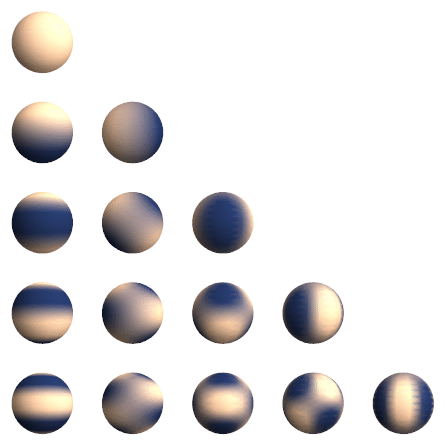
covariance : exponential activation - initial convariance matrix : isotropic Gaussian ( Sphere )
- scheduling : standard exponential decay scheduling
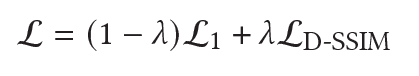
- loss function : L1 + D-SSIM
5.2 Adaptive Control of Gaussians
initialization
: sparse points from SfM
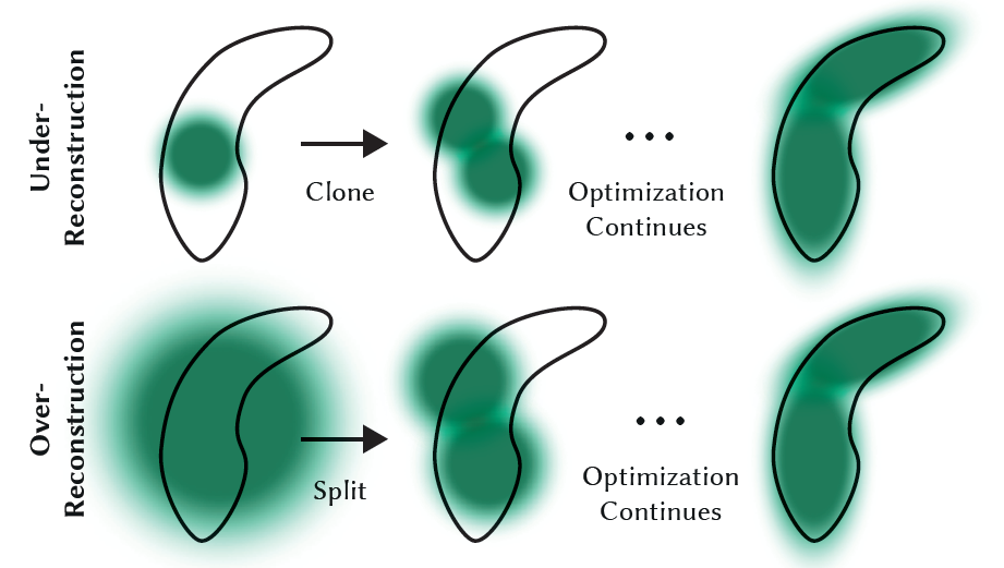
Adaptive Density Control
: adaptively control the number of guassians
- removing Gaussians
: remove gaussians with α less than a threshold 𝜖𝛼 every 100 iterations (almost transparent) - populating Guassians in empty area
case 1) Under reconstruction : missing geometric feature
=> total volume ↑ + the number of gaussians ↑
case 2) Over reconstruction : covering large areas in the scene
=> total volume ↓ + the number of gaussians ↑
- α value
: optimization could get stuck with floaters close to the input cameras.
=> set α close to zero every 3000 iterations -> optimization then increases the α for the Gaussians
Advantage
- remain primitives in Euclidean space
- not require space compaction, warping or projection for distant or large Gaussians
6. Fast differentiable rasterizer for gaussians
final goal : fast overall rendering and fast sorting to allow approximate α-blending
a tile-based rasterizer
- software rasterization approach
- pre-sort primitives for entire image at a time
- efficient backpropagation
- memory : constant per pixel
- fully differentiable
Rasterization Algorithm
function Rasterize(𝑤, ℎ, 𝑀, 𝑆, 𝐶, 𝐴, 𝑉 )
	CullGaussian(𝑝, 𝑉 ) ⊲ Frustum Culling
	𝑀′, 𝑆′ ←ScreenspaceGaussians(𝑀, 𝑆, 𝑉 ) ⊲ Transform
	𝑇 ←CreateTiles(𝑤, ℎ)
	𝐿, 𝐾 ←DuplicateWithKeys(𝑀′, 𝑇 ) ⊲ Indices and Keys
	SortByKeys(𝐾, 𝐿) ⊲ Globally Sort
	𝑅 ←IdentifyTileRanges(𝑇 , 𝐾)
	𝐼 ← 0 ⊲ Init Canvas
	for all Tiles 𝑡 in 𝐼 do
		for all Pixels 𝑖 in 𝑡 do
			𝑟 ←GetTileRange(𝑅, 𝑡 )
			𝐼 [𝑖] ←BlendInOrder(𝑖, 𝐿, 𝑟 , 𝐾, 𝑀′, 𝑆′, 𝐶, 𝐴)
		end for
	end for
	return 𝐼
end function
7. Implementation, results and evaluation
7.1. Implementation
- python (pytorch)
- custom CUDA kernels for rasterization
- NVIDIA CUB sorting routines (Radix Sort)
- interactive viewer (using SIBR)
- source code : https://github.com/graphdeco-inria/gaussian-splatting
GitHub - graphdeco-inria/gaussian-splatting: Original reference implementation of "3D Gaussian Splatting for Real-Time Radiance
Original reference implementation of "3D Gaussian Splatting for Real-Time Radiance Field Rendering" - graphdeco-inria/gaussian-splatting
github.com
optimization details
- lower resolution (1/4 times) -> upsample(250 iters) -> upsample(500iters) -> high resolution
=> improve stability - SH(Spherical Harmonics) coefficient optimization
7.2. Results and Evalution
Results
- tested on 13 real scenes
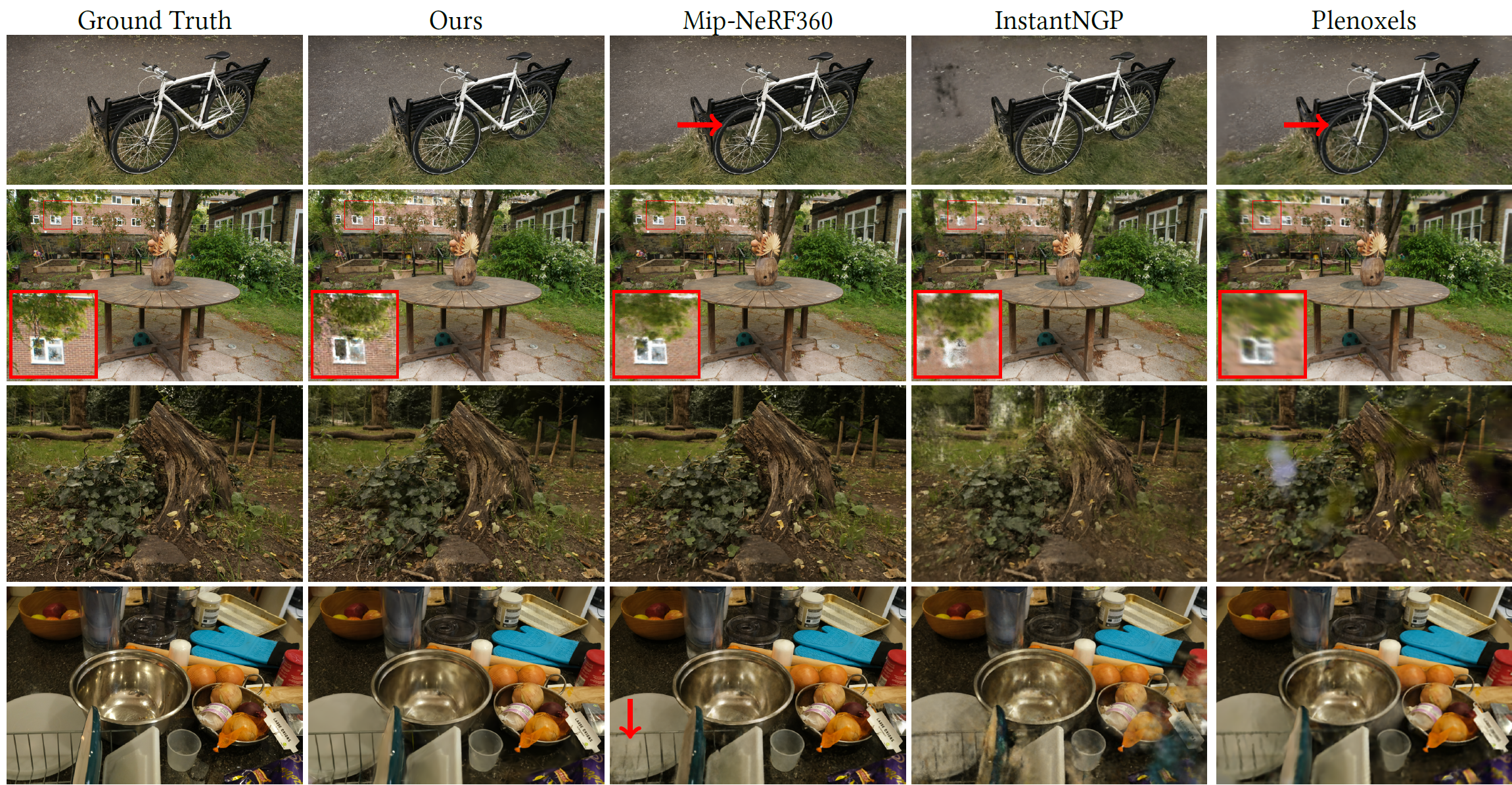
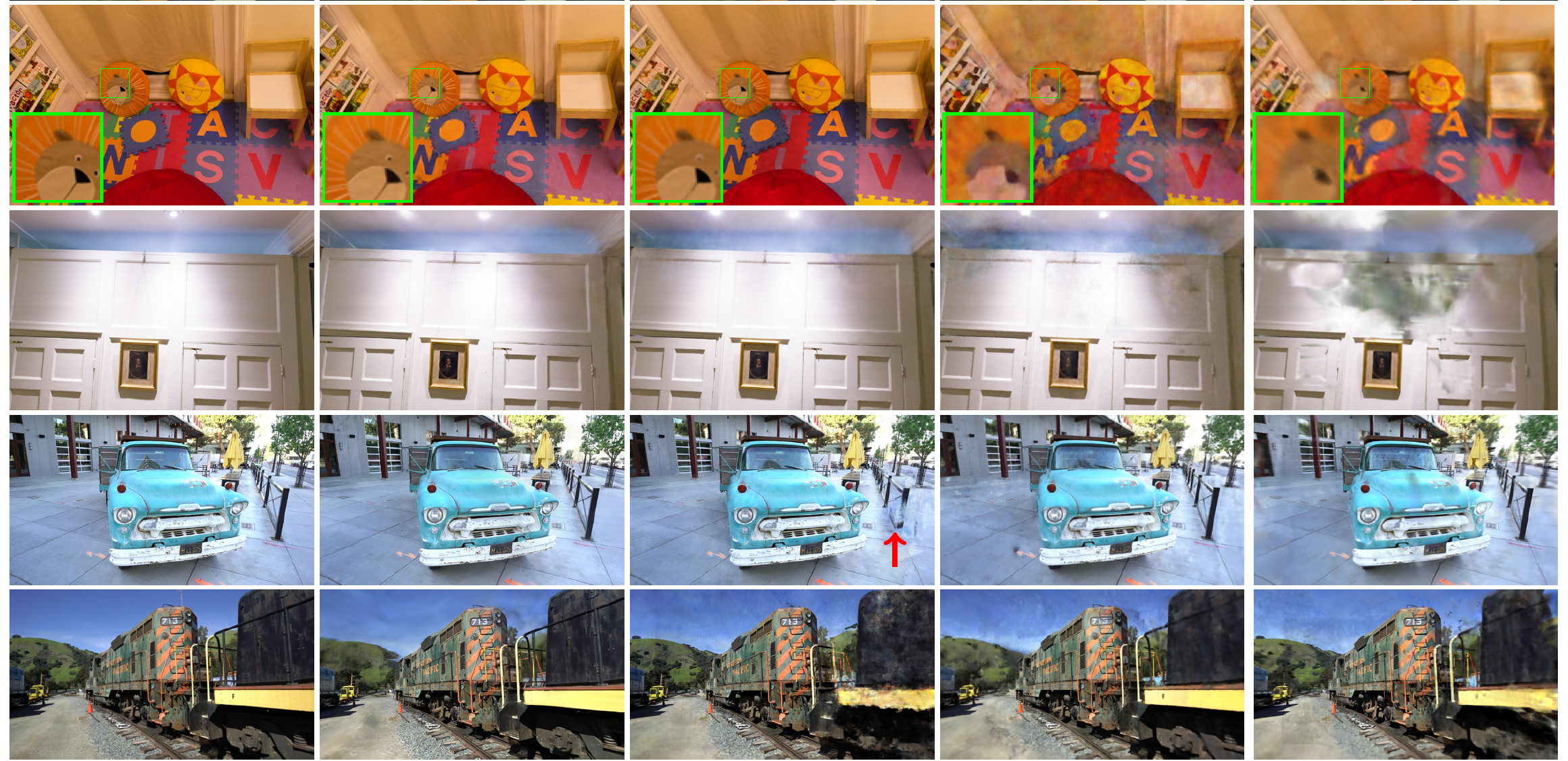
- Real-World Scenes
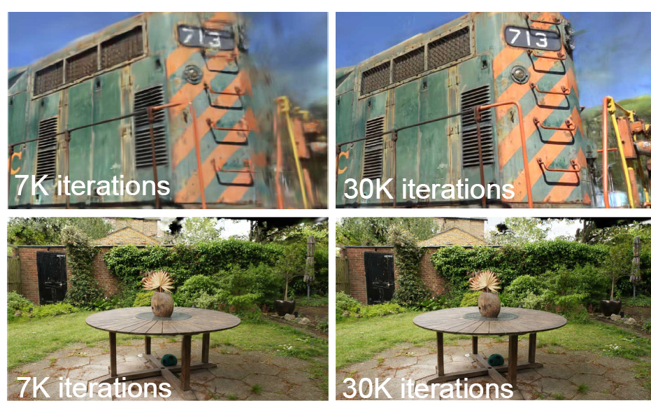
ours : quality at 7K iterations is already good
- Synthetic Bounded Scenes
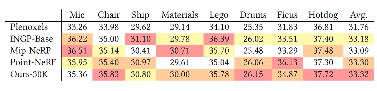
- Compactness
anisotroopic Gaussians are capable of modelling with a lower number of parameters
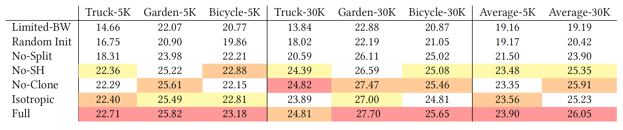
7.3. Ablations
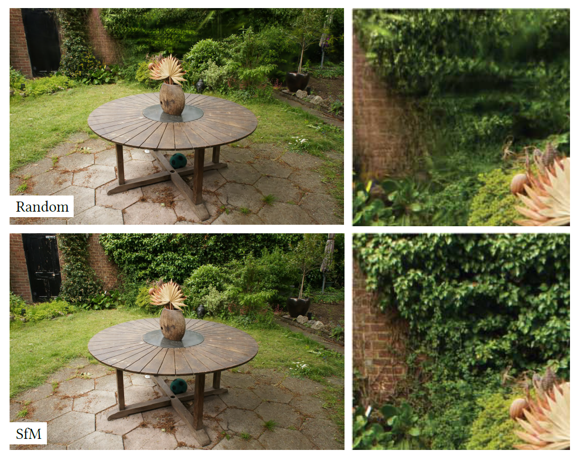
- Initialization with SfM points (random vs SfM)
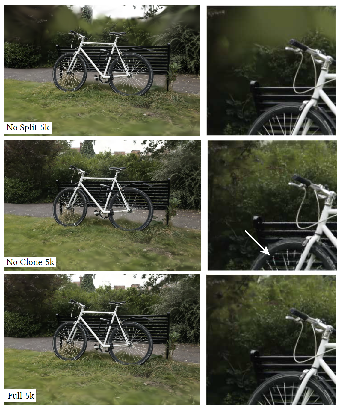
- Densification (clone vs split)
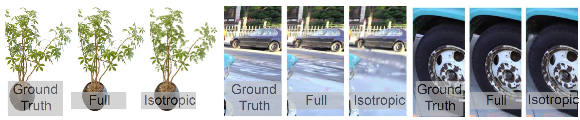
- anisotropic covariance
- spherical harmonics
7.4. Limitation
- popping artifacts : have popping artifacts due to trivial rejection of gaussian
- simple visibility algorithm : may suddenly switching depth/blending order
- same hyperparameters for our full evaluation
- not apply any regularization
- memory consumption is significantly higher
8. Discussion and conclusions
- presented the first real-time rendering solution for radiance fields, with rendering quality that matches the best expensive previous method, with training times competitive with the fastest existing solutions.
'Computer Science > AI' 카테고리의 다른 글
| [3DGS] A Survey on 3D Gaussian Splatting (0) | 2025.03.08 |
|---|---|
| [Nerf] Nerf : Representing Scenes as Neural Radiance Fields for View Synthesis (0) | 2025.03.05 |
| [3DGS] gaussian function - N-dim gaussian (0) | 2025.02.07 |
| [3DGS] Gaussian function - 1D gaussian (0) | 2025.02.07 |
| [AI] 컴퓨터 비전 - 지역 특징 (모라벡, 해리스, SIFT) (1) | 2024.04.21 |