[3DGS] SplaTAM: Splat, Track & Map 3D Gaussians for Dense RGB-D SLAM

Paper Information

• Title : SplaTAM: Splat, Track & Map 3D Gaussians for Dense RGB-D SLAM
• Journal : CVPR 2024
• Date : Apr, 2024 (v3)
• Author :  Nikhil Keetha et al.

 

https://openaccess.thecvf.com/content/CVPR2024/html/Keetha_SplaTAM_Splat_Track__Map_3D_Gaussians_for_Dense_RGB-D_CVPR_2024_paper.html

CVPR 2024 Open Access Repository

 

 

---

 

Abstract

Dense SLAM

• Crucial for robotics.
• Current methods are limited by non-volumetric or implicit representations.

Main Method: SplaTAM

• Enables high-fidelity reconstruction from a single unposed RGB-D camera.
• Provides a simple online tracking and mapping system.
• Utilizes a silhouette mask for improved accuracy.

Results

• Achieves fast rendering and dense optimization.
• Delivers 2× better performance in camera pose estimation, map construction, and novel-view synthesis.

 

 

1. Introduction

SLAM : estimating the poose of visioonn sensor and map of the environment

During past 30 decades, main research of SLAM => map representation

various map representation

• sparse representation
• dense representation
• neural scene representation

 

In terms of dense visual SLAM, the most successful handcrafted represenatations are points, surfels/flats, and signed distance fields.

tracking explicit representations' shortcoming
1) availabiltiy of rich 3D geometrc features and high-framerate captures
2) only reliably explain the observed parts of the scene

=> leads to arise NeRF SLAM algorithm

 

NeRF SLAM
Advantage : high-fidelity global map & image reconstruction, capture dense photometric information
Disadvantage : computationally inefficient, not easy to edit, not model spatial geometry explicitly, catastrophic forgetting

=> How can design better using explicit volumetric representation? : radiance field based on 3D Guassians

 

The benefits of SplaTAM

• fast rendering and rich optimization 
  : can be rendered at speeds up to 400FPS
  
  key of increasing of speed : rasterization of 3D primitives
  1) removal of view-dependent appearance
  2) use of isotropic Gaussians
  3) dense photometric loss for SLAM
  
  
• Maps with explicti spatial extent
  spatial frontier of the exiting map : can identify a new image frame's location by rendering a silhouette
  (This crucial for camera tracking)
• Explicit map
  simply increase the map capacity by adding more Gaussians.
  explicit volumetric representation -> allow to edit parts of the scene & render photo-realistic images 
• Direct Gradient flow to parameters
  this enables fast optimization

 

SOTA for camera pose estimation, map estimaton and novel-view synthesis

 

2. Related Work

2.1. Traditional approaches to dense SLAM

a variety of representations

• 2.5D images
• signed-distance functions
• gaussian mixture moodels
• cirular surfels

However, 2D surfels are discontinuous -> no differentiable.

=> we use voulmetric scene representations in the form of 3D Gaussians (continuous)

 

2.2. Pretrained neural network representations

This approaches range from directly integrating depth predictions

 

2.3. Implicit Scene Representations

• iMAP : first performed both tracking and mapping using neural impliciti representations
• NICE-SLAM : use of hierarchical multi-feature grids
• Point-SLAM : perform volumetric rendering with feature interpolation

However, implict representations limits efficiency

=> we use explicit volumetric radiance model 

 

2.4. 3D Gaussian splatting

3D Guassians : promising 3D scene representation 

In model dynamic scene : require that each input frame has an accurately known with 6-DOF motion

=> we removes this constraints

 

3. Method

SplaTAM : the first dense RGB-D SLAM soluction to use 3D Guassian Splatting

3.1. Guassian Map Representation

Guassan : ( c, µ, o, r )

Eq.1

color : c = (r, g, b) ,
center position : µ ∈ R^3, 
radius : r
opacity : o ∈ [0,1].

using only view-dependent color and forcing Gaussians to be isotropic

 

3.2.  Differentiable Rendering via Splatting

core of our approach : render high-fidelity color, depth, silhouette images from our Gaussian Map in a differentiable way

1. rendered color of pixel p = (u, v)

• f_i(p) : computed as Eq.1
• µ , r : the splatted D Gaussian in pixel-space

• K : (known) camera intrinsic matrix
• E_t : extrinsic matrix capturing the rotation and translation
• f : focal length
• d : depth of i th Gaussian

 

2. rendered depth of pixel p = (u, v)

3. silhouete image of pixel p = (u, v)

 

 

3.3. SLAM System

fitted frames : 1 to t
new RGB-D frames : t+1

1. Camera tracking : minimize image and depth reconstruction error
2. Gaussian Densification : add new guassians to the map based on the rendered silhouette and input depth
3. Map Update : given the frame 1 to t_1, update parameters of all the Gaussians by minimizing error

 

3.4. Initialization

(In first frame)

1. tracking : set is skipped & camera pose is set to identity.
2. densification : silhouette -> empty, add new gaussians
   (depth : unprojection of that pixel depth / o =0.5
   / r = one-pixel radius upon projection b dividing the depth by the focal length)

3.5. Camera Tracking

Camera tracking aims to estimate the camera pose of the current incoming online RGB-D image

 

Camera parameters initialized using the following 

Then, camera pose is updated iteratively by gradient-based optimization and minimize the following loss

L1 loss on both depth and color renders

• apply this loss only sell-optimized parts of the map by using our rendered visibility silhouette
• give value of 1 if there is no GT depth for a pixel

 

3.6. Gaussian Densification

initialize new gaussians in Map at each incoming online frame

Don't add Gaussian if current Gaussians are already accurate

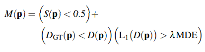
• indicates where the map isn't adequately dense (S <0.5)
• new geometry > the predicted depth & depth error > lamda * median

 

3.7. Gaussian Map Updating

This is equivalent to the classic roblem of fitting a radiance field.

However, there are two modifications

1. warm-start the optimization from recently constructed map
2. do not optimize all previous frames (save each nth frame and select k frames to optimize)

 

+) we add SSIM loss to RGB rendering &  cull useless Gaussian (near 0 opacity or too large)

 

4. Experimental Setup

4.1. Datasets and Evaluation Settings

• datasets : ScanNet++, Replica, TUM-RGBD, ScanNet
• methods : Point-SLAM, NBICE-SAM 

4.2. Evaluation Metrics

• PSNR
• SSIM
• LPIPS
• ATE RMSE (average absolute trajectory error) fr camera pose estimation

4.3. Baselines

main baseline method we compare : Point-SLAM (previous SOTA)

• older dense SLAM  approaches : NICE-SLAM, Vox-FUsion, ESLAM
• traditional SLAM : Kintinuous, ElasticFusion, ORB-SLAM2, DROID-SLAM, ORB-SLAM3

 

5. Results & Discussion

5.1. Camera Pose Estimatiion Results

Overall these camera pose estimation results are extremely promising and show off the strengths of our SplaTAM method.

 

5.2. Rendering Quality Results

 

Our approach acheives a good novel-view synthesis result.

 

Our methods achieve visually excellent results over both scenes for both novel and training view.

 

5.3. Color and Depth Loss Ablation

 

5.4. Camera Tracking Ablation

 

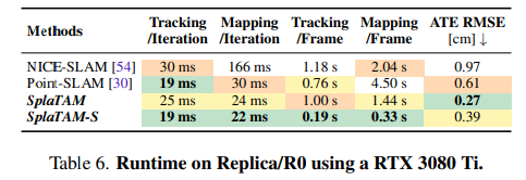
5.5. Runtime Comparison

 

5.6. Limitations & Future work

Limitation

• sensitiviy to motion blur, large depth noise, and aggressive rotation

Future work

• can be scaled up to large-scale scenes through efficient representations
• remove dependencies that require known camera intrinsic

 

 

6. Conclusion

SplaTAM : a novel SLAM system that leverages 3D Gaussians as its underlying map representation to enbable fast renderingand dense optimization

=> achieve SOTA in camera pose estimation, scene reconstruction and novel-view snthesis